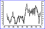
Figure: Naïve X11-trend for the unemployment rate, (%) by month, in a selected region. key: joined dots = original series, bold = fitted trend
As indicated above, users are frequently interested in the LFS data as time-series. They are looking for underlying directions of movement within the series. The month-to-month movement in original data is of little interest in this regard. Volatility in the figures results from seasonal effects, such as new job-seekers hitting the market in December. Interpretation of underlying growth or decline is facilitated by modelling these seasonal effects and removing them from the series. As well as seasonality, there is also volatility associated with irregular influences in the statistics, including sampling and non-sampling error. The effects of the irregular can also be removed by fitting a smoothing-filter to the data, to yield smoothed seasonally-adjusted data. This works well at State and National levels.

Figure:
Naïve X11-trend for the unemployment rate, (%) by month, in a selected region.
key: joined dots = original series, bold = fitted trend
As well as State and National-level estimates, the ABS currently releases estimates of the unemployment-rate and participation-rate from its Labour Force Survey, for each of 64 regions that cover Australia. Given the small sample-sizes at this level, sampling errors in each region are large, leading to strong volatility in the data.
However another concern at this level is the degree of auto-correlation, due to the rotating-panel nature of the sample. In these small-sample cases, it is possible for a very atypical area to be rotated into sample, leading to high or low estimates of employment or unemployment at that geographic level, over a period of months. These auto-correlations induce spurious trend-cycles in the smoothed data, which need to be separated from the trend of the population values when the latter is of interest. These cycles are not identified or removed within the standard seasonal-adjustment packages commonly used for trend estimation.

Figure:
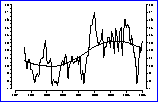
New trend for unemployment rate (%) by month, in a selected region.
key: joined dots = original series, bold = fitted trend
This is illustrated in the graphs for a particular regional unemployment series, shown as figures 3 and 4. The trend using a naive application of the standard ( X11) method is shown superimposed on the original data. A feature of this trend curve is a large number of turning-points -- these are actually due to auto-correlated sampling error.
As part of a research project, auto-correlations of the sampling-errors over time, have been estimated from knowledge of the 8 distinct rotation-panel estimates. These are used to model the sampling-error structure. Such a model can be combined with a model for the unemployment-series population values, to extract separately particular components attributable to trend, seasonal, irregular and sampling-error. The results of this analysis, for the same data as presented in figure 3, is shown in figure 4. Simulations demonstrate that trends produced using this method actually give much more accurate estimates of the true activity within the population.