
MieSolver
An Object Oriented Mie Series Software
AboutWave Scattering by CylindersMieSolver is a simple and easy to use Matlab program for simulating acoustic and electromagnetic wave propagation through a configuration of one or more non-identical circular cylinders. Multiple scattering effects are fully simulated. MieSolver is based on the Mie Series solution of the wave propagation model. For full details see the accompanying paper. MieSolver supports
The object-oriented structure of the software allows mixed configurations of cylinders with the following material properties:
MieSolver implements the following incident waves:
| ||||||||||||||||||||||||||||||||||||||||||||||||||||||||||||||||||||||||||||||||||||||||
LicenseMieSolver is free software: you can redistribute it and/or modify it under the terms of the GNU General Public License as published by the Free Software Foundation, either version 3 of the License, or (at your option) any later version. This program is distributed in the hope that it will be useful, but WITHOUT ANY WARRANTY; without even the implied warranty of MERCHANTABILITY or FITNESS FOR A PARTICULAR PURPOSE. See the GNU General Public License for more details.
If you use this code, please cite the accompanying paper: |
||||||||||||||||||||||||||||||||||||||||||||||||||||||||||||||||||||||||||||||||||||||||
DownloadDownload user manual miesolver_manual.pdf Download all files (including documentation and examples):
|
||||||||||||||||||||||||||||||||||||||||||||||||||||||||||||||||||||||||||||||||||||||||
Contact
|
||||||||||||||||||||||||||||||||||||||||||||||||||||||||||||||||||||||||||||||||||||||||
ExampleWe use MieSolver to simulate scattering of an incident plane wave by two cylinders. The first cylinder has a metal core and a dielectric coating. The second cylinder is metal. (full code).Create the scatterersIn MieSolver all scatterers have a core, to which layers can be added. We setup the first scatterer by first creating a metal core with radius 0.5 and then adding a dielectric layer. The position of the centre of the core is specified using a complex number -1-i to represent (-1,-1). For this example we will use a transverse electric (TE) incident wave so that the metal core has a sound-soft type boundary condition.
Visualise the configurationOnce created we can visualise our configuration of two scatterers..
The result looks like this: 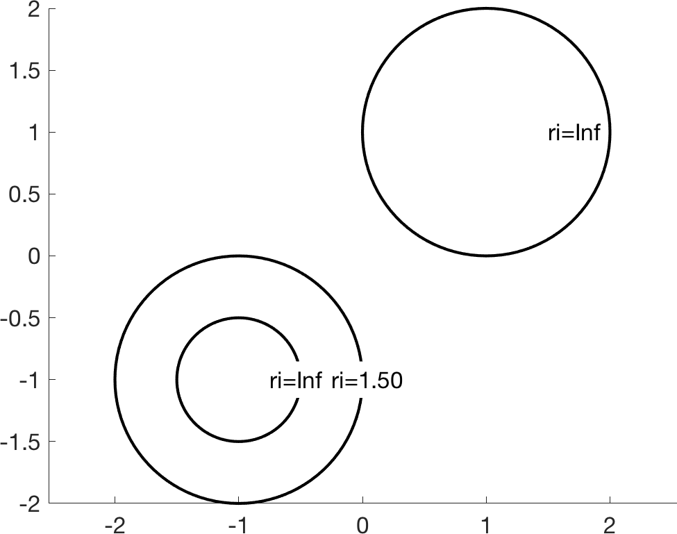
Setup the incident waveWe will use an incident plane wave travelling in the direction (0,1) i.e. with angle pi/2 and wavenumber 5 pi.
Setup and solve the scattering problemNext we setup the MieSolver object that we use to solve the scattering problem. This is where we specify what kind of transmission conditions are to be applied. In this example we use transverse electric (TE) type transmission conditions.
Visualise the total fieldMieSolver has built in methods for quickly visualising the scattered/induced and total fields. The plot region is specified by its bottom left and top right corners.
The result looks like this: 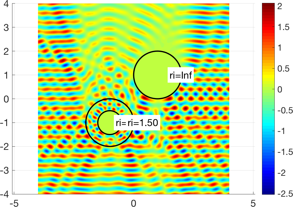
Full codeYou can paste the full code into your Matlab command window.
|